This is part three of my “Notes on ‘Non-linear PCA” blog article series, where I discuss various deep generative modeling techniques. In this section, I am going to discuss diffusion models.
Introduction#
Diffusion models are different kinds of latent variable models compared to VAEs and GANs, and they take inspiration non-equilibrium statistical physics. The main idea behind them is that, given some dataset $\mathbf{X}$, we will repeatedly apply Gaussian noise to each data example $\mathbf{x}^{(i)}$ iteratively until the transformed data example is indistinguishable from noise sampled from the multivariate unit Gaussian. Then, we use a neural network which learns to iteratively undo the previously-applied diffusion steps in order to reconstruct the original example $\mathbf{x}^{(i)}$. Unlike VAEs or GANs, diffusion models are learned with a fixed procedure and the latent variable has high dimensionality; the same dimensionality as the input data, in fact.
Just like before in VAEs, we are interested in finding a distribution over data, $p_\theta(\mathbf{x})$; however, we make the assumption that we have an additional set of latent variables $\mathbf{z} = [\mathbf{z}_1,…,\mathbf{z}_T]$.
The joint distribution of the latents and the observed variable is modelled to follow the Markov assumption:
$$
\begin{align*}
p_\theta(\mathbf{x}, \mathbf{z}_{1:T}) = p_\theta(\mathbf{x} | \mathbf{z}_{1}) \bigg(\prod_{t=1}^{T-1} p_\theta(\mathbf{z}_t | \mathbf{z}_{t+1})\bigg) p_\theta(\mathbf{z}_T)
\end{align*}
$$
Essentially, we have a markov chain of latent variables $\mathbf{z}_i$ that eventually lead up to our observed variable $\mathbf{x}_i.$ These are parametrized using DNNs. This is similar to the VAE setup, but with many multiple latent variable dependencies. Moreover, unlike VAEs, we assume that $\mathbf{x}$ and $\mathbf{z}$ contain the same dimensionality
.
We then see that the marginal likeliood of our data is found by integrating out all of the latent variables:
$$
\begin{align*}
p_\theta(\mathbf{x}) = \int p_\theta(\mathbf{x}, \mathbf{z}_{1:T})d\mathbf{z}_{1:T}
\end{align*}
$$
Now, we will relate this to setup to the diffusion process.
Foward diffusion process#
Similar to VAEs, we are also interested in finding distributions that model the posteriors as follows:
$$
\begin{align}
q_\phi(\mathbf{z}_{1:T}|\mathbf{x}) = q_\phi(\mathbf{z}_1 | \mathbf{x})\bigg(\prod_{i=2}^T q_\phi(\mathbf{z}_t | \mathbf{z}_{t - 1})\bigg)
\end{align}
$$
In VAEs, we’d parametrize these posterior distributions using deep neural networks. However, here, we will formuate them using the following forward Gaussian diffusion process:
$$
\begin{align*}
q_\phi(\mathbf{z}_t | \mathbf{z}_{t-1}) &= \mathcal{N}(\mathbf{z}_t;\sqrt{1-\beta_t}\mathbf{z}_{t-1}, \beta_t\mathbf{I}),
\end{align*}
$$
where $\beta_t \in [0, 1]$ are step sizes controlled by a variance schedule for all $t \in [T],$ and where $\beta_1 < \beta_2 <…<\beta_T.$ Here, we are adding a small amount of Gaussian noise to the our sample in $T$ timesteps. By doing this, we produce a sequence of noisy samples $\mathbf{z}_1,…,\mathbf{z}_T$.
Because each latent $\mathbf{z}_t$
is generated by adding some Gaussian noise to the observed variable $\mathbf{x}$ over $t$ timesteps, it is then natural to instead think each latent variable $\mathbf{z}_t$
as $\mathbf{x}_t$
and of the observed variable as $\mathbf{x}_0$
. Thus, our joint distribution now becomes
$$
\begin{align*}
p_\theta(\mathbf{x}_0, \mathbf{x}_{1:T}) = \bigg(\prod_{t=0}^{T-1} p_\theta(\mathbf{x}_t | \mathbf{x}_{t+1})\bigg) p_\theta(\mathbf{x}_T),
\end{align*}
$$
our marginal likelihood becomes
$$
\begin{align*}
p_\theta(\mathbf{x}_0) = \int p_\theta(\mathbf{x}_0, \mathbf{x}_{1:T})d\mathbf{x}_{1:T},
\end{align*}
$$
our variational posteriors become
$$
\begin{align*}
q_\phi(\mathbf{x}_{1:T}|\mathbf{x}_0) &= \prod_{t=1}^T q_\phi(\mathbf{x}_t|\mathbf{x}_{t-1}),
\end{align*}
$$
and each posterior is modelled by
$$
\begin{align*}
q_\phi(\mathbf{x}_t | \mathbf{x}_{t-1}) &= \mathcal{N}(\mathbf{x}_t;\sqrt{1-\beta_t}\mathbf{x}_{t-1}, \beta_t\mathbf{I}).
\end{align*}
$$
As the noising process goes on, the data sample $\mathbf{x}_0$ gradually loses its distinguishable features as the step $t$ becomes larger and when $T \to \infty$, $\mathbf{x}_T$, it is indistinguishable to a sample drawn from the standard Gaussian distribution.
We can write each $\mathbf{x}_t$ by using the same reparametrization trick used in VAEs:
$$
\begin{align*}
\mathbf{x}_t &= \sqrt{1 - \beta_t} \mathbf{x}_{t-1} + \sqrt{\beta_t} \odot \epsilon,
\end{align*}
$$
where $\epsilon \sim \mathcal{N}(\mathbf{0, \mathbf{1}}).$
Reverse diffusion process#
Ultimately, our goal is to reverse this forward Gaussian diffusion process and sample from $q_\phi(\mathbf{x}_{t-1}|\mathbf{x}_t)$
to create a true example from a Gaussian noise input $\mathbf{x}_T \sim \mathcal{N}(\mathbf{0}, \mathbf{I}).$
Note that
$$
\begin{align*}
q_\phi(\mathbf{x}_{t-1}|\mathbf{x}_t) &= \frac{q_\phi(\mathbf{x}_t | \mathbf{x}_{t-1})q_\phi(\mathbf{x}_{t-1})}{q_\phi(\mathbf{x}_t)}\\
&= \frac{q_\phi(\mathbf{x}_t | \mathbf{x}_{t-1})q_\phi(\mathbf{x}_{t-1})}{\int q_\phi(\mathbf{x}_t, \mathbf{x}_{t+1:T})d\mathbf{x}_{t+1:T}}
\end{align*}
$$
As we can see, the denominator is intractable. However, do note that if $\beta_t$ is small enough, $q_\phi(\mathbf{x}_{t-1}|\mathbf{x}_t)$
, follows a Gaussian distribution; this is a result from the application of stochastic differential equations, and to see more on how this is derived can be found in
.
It turns out that $p_\theta$ can approximate these conditional probabilities in order to run the reverse diffusion process, which can done by setting:
$$
\begin{align*}
p_\theta(\mathbf{x}_{t-1}|\mathbf{x}_t) = \mathcal{N}(\mathbf{x}_{t-1};\mu_{\theta}(\mathbf{x}_t,t),\Sigma_{\theta}(\mathbf{x}_t,t)),
\end{align*}
$$
where $\mu_\theta$ and $\Sigma_\theta$ are neural networks.
Finding the ELBO for training#
We want our model to maximize the log-likelihood of our data; this will be intractable, but this can be approximated using ELBO as in VAEs:
$$
\begin{align*}
&\log p_\theta(\mathbf{x}_0) = \log \int p_\theta(\mathbf{x}_{0},\mathbf{x}_{1:T})d\mathbf{x}_{1:T}\\
&= \log \int q_\phi(\mathbf{x}_{1:T}|\mathbf{x}_0)\frac{p_\theta(\mathbf{x}_{0}, \mathbf{x}_{1:T})}{q_\phi(\mathbf{x}_{1:T}|\mathbf{x}_0)}d\mathbf{x}_{1:T}\\
&= \log \bigg(\mathbb{E}_{q_\phi(\mathbf{x}_{1:T}|\mathbf{x}_0)}\bigg[\frac{p_\theta(\mathbf{x}_{0}, \mathbf{x}_{1:T})}{q_\phi(\mathbf{x}_{1:T}|
\mathbf{x}_0)}\bigg]\bigg)\\
&\geq \mathbb{E}_{q_\phi(\mathbf{x}_{1:T}|\mathbf{x}_0)}\bigg[\log \frac{p_\theta(\mathbf{x}_{0}, \mathbf{x}_{1:T})}{q_\phi(\mathbf{x}_{1:T}|\mathbf{x}_0)}\bigg]\\
&=\mathbb{E}_{q_\phi(\mathbf{x}_{1:T}|\mathbf{x}_0)}\bigg[\log p_\theta(\mathbf{x}_{0}, \mathbf{x}_{1:T}) - \log q_\phi(\mathbf{x}_{1:T}|\mathbf{x}_0) \bigg]\\
&=\mathbb{E}_{q_\phi(\mathbf{x}_{1:T}|\mathbf{x}_0)}\bigg[\log\bigg( \bigg(\prod_{t=0}^{T-1} p_\theta(\mathbf{x}_t | \mathbf{x}_{t+1})\bigg) p_\theta(\mathbf{x}_T)\bigg) - \log \bigg( \prod_{t=1}^T q_\phi(\mathbf{x}_t|\mathbf{x}_{t-1})\bigg)\bigg]\\
&=\mathbb{E}_{q_\phi(\mathbf{x}_{1:T}|\mathbf{x}_0)}\bigg[\log p_\theta(\mathbf{x}_T) + \log \sum_{t= 0}^{T-1} p_\theta(\mathbf{x}_t|\mathbf{x}_{t+1}) - \sum_{t=1}^T \log q_\phi(\mathbf{x}_t|\mathbf{x}_{t-1})\bigg]\\
&=\mathbb{E}_{q_\phi(\mathbf{x}_{1:T}|\mathbf{x}_0)}\bigg[\log p_\theta(\mathbf{x}_0 | \mathbf{x}_1) + \sum_{t=1}^{T-1} \bigg(\log p_\theta(\mathbf{x}_t | \mathbf{x}_{t+1})-\log q_\theta(\mathbf{x}_t | \mathbf{x}_{t-1})\bigg) \\
&+ \log p_\theta(\mathbf{x}_T) - \log q_\phi(\mathbf{x}_T | \mathbf{x}_{T-1})\bigg]\\
&= \mathcal{L}(\mathbf{x}; \theta, \phi).
\end{align*}
$$
We can write this ELBO in terms of KL-divergences:
$$
\begin{align*}
&\mathcal{L}(\mathbf{x}; \theta, \phi) = \mathbb{E}_{q_\phi(\mathbf{x}_{1:T}|\mathbf{x}_0)} [\log p_\theta(\mathbf{x}_0 \vert \mathbf{x}_1)]\\
& - \sum_{t=1}^T \mathbb{E}_{q_\phi(\mathbf{x}_{-t}|\mathbf{x}_0)} [D_\text{KL}(q_\phi(\mathbf{x}_{t} \vert \mathbf{x}_{t-1}) \parallel p_\theta(\mathbf{x}_{t} \vert\mathbf{x}_{t+1}))]\\
&-\mathbb{E}_{q_\phi(\mathbf{x}_{-T}|\mathbf{x}_0)} [D_\text{KL}(q(\mathbf{x}_T \vert \mathbf{x}_{T-1}) \parallel p_\theta(\mathbf{x}_T))],
\end{align*}
$$
where $q_\phi(\mathbf{x}_{-t}|\mathbf{x}_0)$ denotes the posterior distribution excluding $\mathbf{x}_t$. We can then integrate out superfluous dependencies in the expectation to see that:
$$
\begin{align*}
&\mathcal{L}(\mathbf{x}; \theta, \phi) = \mathbb{E}_{q_\phi(\mathbf{x}_{1}|\mathbf{x}_0)} [\log p_\theta(\mathbf{x}_0 \vert \mathbf{x}_1)]\\
& - \sum_{t=1}^T \mathbb{E}_{q_\phi(\mathbf{x}_{t-1,t+1}|\mathbf{x}_0)} [D_\text{KL}(q_\phi(\mathbf{x}_{t} \vert \mathbf{x}_{t-1}) \parallel p_\theta(\mathbf{x}_{t} \vert\mathbf{x}_{t+1}))]\\
&-\mathbb{E}_{q_\phi(\mathbf{x}_{T-1}|\mathbf{x}_0)} [D_\text{KL}(q(\mathbf{x}_T \vert \mathbf{x}_{T-1}) \parallel p_\theta(\mathbf{x}_T))],
\end{align*}
$$
Note that each of the KL-divergence terms inside the loss are the KL-divergence between two gaussians, so each of them can be rewritten as L2-loss with respect to the means.
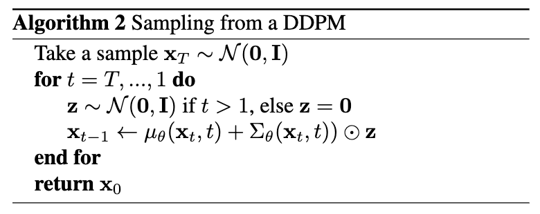
Given this, we outline the training algorithm in Algorithm 1 and the sampling algorithm in Algorithm 2.

Improving DDPMs#
We define $\alpha_t = 1 - \beta_t$
, and we also define $\bar{\alpha}_t = \prod_{i=1}^t \alpha_i$
. Recall from the reparametrization trick that
$$
\begin{align*}
\mathbf{x}_t
&= \sqrt{1 - \beta_t}\mathbf{x}_{t-1} + \sqrt{\beta_t}\boldsymbol{\epsilon}_{t-1},\\
\end{align*}
$$
where
$\mathbf{\epsilon}_{t-1} \sim \mathcal{N}(\mathbf{0}, \mathbf{I})$
. We can then expand out the expression to find that
$$
\begin{align*}
\mathbf{x}_t
&= \sqrt{1 - \beta_t}\mathbf{x}_{t-1} + \sqrt{\beta_t}\boldsymbol{\epsilon}_{t-1}\\
&= \sqrt{\alpha_t}\mathbf{x}_{t-1} + \sqrt{1 - \alpha_t}\boldsymbol{\epsilon}_{t-1}\\
&= \sqrt{\alpha_t}(\sqrt{\alpha_{t-1}}x_{t-2} + \sqrt{1 - \alpha_{t-1}} \epsilon_{t-2}) + \sqrt{1 - \alpha_t} \epsilon_{t-1}\\
&= \sqrt{\alpha_t \alpha_{t-1}} \mathbf{x}_{t-2} + \underbrace{\sqrt{\alpha_t(1 - \alpha_{t-1})}\epsilon_{t-2} + \sqrt{1 - \alpha_t}\epsilon_{t-1}}_{\text{merging 2 gaussians } \mathcal{N}(0, \sigma_1^2I) \text{ and } \mathcal{N}(0, \sigma_2^2I) \text{ creates } \mathcal{N}(0, \sigma_1^2 + \sigma_2^2I)}\\
&= \sqrt{\alpha_t \alpha_{t-1}} \mathbf{x}_{t-2} + \underbrace{\sqrt{\alpha_t(1 - \alpha_{t-1}) + (1 - \alpha_t)}}_{\text{square root of variance of merged gaussian}}\bar{\epsilon}_{t-2}\\
&= \sqrt{\alpha_t \alpha_{t-1}} \mathbf{x}_{t-2} + \sqrt{1 - \alpha_t \alpha_{t-1}} \bar{\boldsymbol{\epsilon}}_{t-2} \\
&= \dots \\
&= \sqrt{\bar{\alpha}_t}\mathbf{x}_0 + \sqrt{1 - \bar{\alpha}_t}\boldsymbol{\epsilon} \\
q(\mathbf{x}_t \vert \mathbf{x}_0) &= \mathcal{N}(\mathbf{x}_t; \sqrt{\bar{\alpha}_t} \mathbf{x}_0, (1 - \bar{\alpha}_t)\mathbf{I})
\end{align*}
$$
This is a really neat property, because this means that in order to calculate noise at specific time-step, we won’t need to perform multiple noising iterations, we can just do it all in one go!
It also actually turns out that when we condition the reverse process on the input as well, meaning $q_\phi(\mathbf{x}_{t-1} | \mathbf{x}_t, \mathbf{x}_0)$
, we can obtain a tractable closed-form solution for a Gaussian. To start, we must first see that
$$
\begin{align*}
q_\phi(\mathbf{x}_{t-1}|\mathbf{x}_t,\mathbf{x}_0) &= \frac{q_\phi(\mathbf{x}_{t-1},\mathbf{x}_t,\mathbf{x}_0)}{q_\phi(\mathbf{x}_t,\mathbf{x}_0)} = \frac{q_\phi(\mathbf{x}_t | \mathbf{x}_{t-1}, \mathbf{x}_0) q(\mathbf{x}_{t-1}, \mathbf{x}_0)}{q_\phi(\mathbf{x}_t,\mathbf{x}_0)}\\
&= \frac{q(x_t | x_{t-1}, x_0) q(x_{t-1} | x_0) q(x_0)}{q(x_t, x_0)}\\
&= \frac{q(x_t | x_{t-1}, x_0) q(x_{t-1} | x_0)}{q(x_t | x_0)} \cdot \frac{q(x_0)}{q(x_0)}\\
&= \frac{q(x_t | x_{t-1}, x_0) q(x_{t-1} | x_0)}{q(x_t | x_0)}.
\end{align*}
$$
Recall that
$$
\begin{align*}
q(x_t | x_{t-1}, x_0) &= q(x_t | x_{t-1}) = \mathcal{N}(\mathbf{x}_t;\sqrt{\alpha_t}\mathbf{x}_{t-1}, \beta_t\mathbf{I})\\
q(x_{t-1} | x_0) &= \mathcal{N}(\mathbf{x}_{t-1}; \sqrt{\bar{\alpha}_{t-1}} \mathbf{x}_0, (1 - \bar{\alpha}_{t-1})\mathbf{I})\\
q(\mathbf{x}_t \vert \mathbf{x}_0) &= \mathcal{N}(\mathbf{x}_t; \sqrt{\bar{\alpha}_t} \mathbf{x}_0, (1 - \bar{\alpha}_t)\mathbf{I})
\end{align*}
$$
The first equation holds because we consider the noising process to be a markov process.
Let
$$
\begin{align*}
c_1 &= |2\pi \beta_t \mathbf{I}|^{-\frac{1}{2}}\\
c_2 &= |2\pi (1 - \bar{\alpha}_{t-1}) \mathbf{I}|^{-\frac{1}{2}}\\
c_3 &= |2\pi (1 - \bar{\alpha}_{t}) \mathbf{I}|^{-\frac{1}{2}}\\
\end{align*}
$$
We can then see that
$$
\begin{align*}
q_\phi(\mathbf{x}_{t-1}|\mathbf{x}_t,\mathbf{x}_0) &= \frac{c_1c_2}{c_3} \exp\bigg\{-\frac{1}{2}\bigg(\frac{(x_t - \sqrt{\alpha_t}x_{t-1})^2}{\beta_t} + \frac{(x_{t-1} - \sqrt{\bar{\alpha}_{t-1}}x_0)^2}{1 - \bar{\alpha}_{t}} - \frac{(x_{t} - \sqrt{\bar{\alpha}_{t}}x_0)^2}{1 - \bar{\alpha}_{t}}\bigg)\bigg\}\\
&= \frac{|2\pi \beta_t \mathbf{I}|^{-\frac{1}{2}} \cdot |2\pi (1 - \bar{\alpha}_{t-1}) \mathbf{I}|^{-\frac{1}{2}}}{|2\pi (1 - \bar{\alpha}_{t}) \mathbf{I}|^{-\frac{1}{2}}} \exp \bigg\{-\frac{1}{2}\bigg(\bigg(\frac{\alpha_t}{\beta_t} + \frac{1}{1 - \bar{\alpha}_{t-1}}\bigg)x_{t-1}^2 - \bigg(\frac{2\sqrt{\alpha_t}}{\beta_t}x_t + \\
&\frac{2\sqrt{\bar{\alpha}_{t-1}}}{1 - \bar{\alpha}_{t-1}}x_0\bigg)x_{t-1} +\bigg(\frac{1}{\beta_t} - \frac{1}{1 - \bar{\alpha}_t}\bigg)x_t^2 + \bigg(\frac{2 \sqrt{\bar{\alpha}_t}}{1 - \bar{\alpha}_t}\bigg)x_0x_t + \bigg(\frac{\bar{\alpha}_{t-1}}{1 - \bar{\alpha}_{t-1}} - \frac{\bar{\alpha}_t}{1 - \bar{\alpha}_t}\bigg)x_0^2\bigg)\bigg\}\\
&= \bigg| 2\pi \bigg( \frac{(1 - \bar{\alpha}_{t-1})\beta_t}{1 - \bar{\alpha}_t} \bigg) \mathbf{I}\bigg|^{-\frac{1}{2}} \exp \bigg\{-\frac{1}{2} \cdot \frac{1 - \bar{\alpha}_t}{(1 - \bar{\alpha}_{t-1})\beta_t}\bigg(x_{t - 1} - \bigg( \frac{\sqrt{\alpha_t}(1 - \bar{\alpha}_{t-1})}{1 - \bar{\alpha}_t} \mathbf{x}_t + \frac{\sqrt{\bar{\alpha}_{t-1}}\beta_t}{1 - \bar{\alpha}_t} \mathbf{x}_0\bigg) \bigg)^2\bigg\}\\
\end{align*}
$$
Thus, we can then see that
$$
q_\phi(\mathbf{x}_{t-1}|\mathbf{x}_t,\mathbf{x}_0) = \mathcal{N}(x_{t-1}; \tilde{\mu}(x_t, x_0), \tilde{\beta}_t\mathbf{I}),
$$
where
$$
\begin{align*}
&\tilde{\mu}(x_t, x_0) = \frac{\sqrt{\alpha_t}(1 - \bar{\alpha}_{t-1})}{1 - \bar{\alpha}_t} \mathbf{x}_t + \frac{\sqrt{\bar{\alpha}_{t-1}}\beta_t}{1 - \bar{\alpha}_t} \mathbf{x}_0,\\
&\tilde{\beta}_t = \frac{(1 - \bar{\alpha}_{t-1})\beta_t}{1 - \bar{\alpha}_t}.\\
\end{align*}
$$
This finding is significant because it allows us to speed up the training process, which we will see how in a bit.
We can rewrite the loss as
$$
\begin{align*}
\mathcal{L}(\mathbf{x}; \theta, \phi) &= \mathbb{E}_{q_\phi(\mathbf{x}_{1:T}|\mathbf{x}_0)} [\log p_\theta(\mathbf{x}_0 \vert \mathbf{x}_1)] - \sum_{t=1}^T \mathbb{E}_{q_\phi(\mathbf{x}_{-t}|\mathbf{x}_0)} [D_\text{KL}(q_\phi(\mathbf{x}_{t} \vert \mathbf{x}_{t-1}) \parallel p_\theta(\mathbf{x}_{t} \vert\mathbf{x}_{t+1}))]\\
&-\mathbb{E}_{q_\phi(\mathbf{x}_{-T}|\mathbf{x}_0)} [D_\text{KL}(q(\mathbf{x}_T \vert \mathbf{x}_{T-1}) \parallel p_\theta(\mathbf{x}_T))]\\
&=\mathbb{E}_{q_\phi(\mathbf{x}_{1:T}|\mathbf{x}_0)}\bigg[\log p_\theta(\mathbf{x}_0 | \mathbf{x}_1) + \sum_{t=1}^{T-1} \bigg(\log p_\theta(\mathbf{x}_t | \mathbf{x}_{t+1})-\log q_\phi(\mathbf{x}_t | \mathbf{x}_{t-1})\bigg) \\
&+ \log p_\theta(\mathbf{x}_T) - \log q_\phi(\mathbf{x}_T | \mathbf{x}_{T-1})\bigg]\\
&=\mathbb{E}_{q_\phi(\mathbf{x}_{1:T}|\mathbf{x}_0)}\bigg[\log p(x_T) + \sum_{t=1}^T \log p(x_{t-1} | x_t) - \log q(x_t | x_{t-1})\bigg]\\
&=\mathbb{E}_{q_\phi(\mathbf{x}_{1:T}|\mathbf{x}_0)}\bigg[\log p(x_T) + \sum_{t=2}^T \bigg(\log p(x_{t-1} | x_t) - \log q(x_t | x_{t-1})\bigg) + \log \frac{p(x_0|x_1)}{q(x_1|x_0)}\bigg]\\
&=\mathbb{E}_{q_\phi(\mathbf{x}_{1:T}|\mathbf{x}_0)}\bigg[\log p(x_T) + \sum_{t=2}^T \bigg(\log \frac{p(x_{t-1} | x_t)}{q(x_t | x_{t-1})}\bigg) + \log \frac{p(x_0|x_1)}{q(x_1|x_0)}\bigg]\\
&=\mathbb{E}_{q_\phi(\mathbf{x}_{1:T}|\mathbf{x}_0)}\bigg[\log p(x_T) + \sum_{t=2}^T \bigg(\log \frac{p(x_{t-1} | x_t)}{q(x_{t-1} | x_t, x_0)} \cdot \frac{q(x_{t-1}|x_0)}{q(x_t|x_0)}\bigg) + \log \frac{p(x_0|x_1)}{q(x_1|x_0)}\bigg]\\
&=\mathbb{E}_{q_\phi(\mathbf{x}_{1:T}|\mathbf{x}_0)}\bigg[\log p(x_T) + \sum_{t=2}^T \bigg(\log \frac{p(x_{t-1} | x_t)}{q(x_{t-1} | x_t, x_0)}\bigg)\\
&+ \sum_{t=2}^T \bigg(\log q(x_{t-1}|x_0) - \log q(x_t|x_0)\bigg) + \log \frac{p(x_0|x_1)}{q(x_1|x_0)}\bigg]\\
&=\mathbb{E}_{q_\phi(\mathbf{x}_{1:T}|\mathbf{x}_0)}\bigg[\log p(x_T) + \sum_{t=2}^T \bigg(\log \frac{p(x_{t-1} | x_t)}{q(x_{t-1} | x_t, x_0)} \bigg)+ \log q(x_1|x_0) - \log q(x_T | x_0) + \log \frac{p(x_0 | x_1)}{q(x_1 | x_0)}\bigg]\\
&=\mathbb{E}_{q_\phi(\mathbf{x}_{1:T}|\mathbf{x}_0)}\bigg[\log \frac{p(x_T)}{q(x_T|x_0)} + \sum_{t=2}^T \bigg(\log \frac{p(x_{t-1} | x_t)}{q(x_{t-1} | x_t, x_0)} \bigg)+ \log p(x_0 | x_1)\bigg]\\
&=\mathbb{E}_{q_\phi(\mathbf{x}_{1:T}|\mathbf{x}_0)}\bigg[\log \frac{p(x_T)}{q(x_T|x_0)} + \sum_{t=2}^T \bigg(\log \frac{p(x_{t-1} | x_t)}{q(x_{t-1} | x_t, x_0)} \bigg)+ \log p(x_0 | x_1)\bigg]\\
&= \mathbb{E}_{q_\phi(\mathbf{x}_{-T}|\mathbf{x}_0)}\bigg[ -D_{\text{KL}}(q(x_T|x_0)||p(x_T)) \bigg] + \sum_{t=2}^T \mathbb{E}_{q_\phi(\mathbf{x}_{1:T}|\mathbf{x}_0)}\bigg[-D_{\text{KL}}(q(x_{t-1}|x_t,x_0)||p(x_{t-1}|x_t))\bigg]\\
&+ \mathbb{E}_{q_\phi(\mathbf{x}_{1:T}|\mathbf{x}_0)}\bigg[ \log p(x_0 | x_1)\bigg]\\
\end{align*}
$$
When we want to minimize the loss instead of maximizing this quantity, we then instead define it as
$$
\begin{align*}
\mathcal{L}(\mathbf{x}; \theta, \phi)&=\mathbb{E}_{q_\phi(\mathbf{x}_{-T}|\mathbf{x}_0)}\bigg[ \underbrace{D_{\text{KL}}(q(x_T|x_0)||p(x_T))}_{L_T} \bigg] + \sum_{t=2}^T \mathbb{E}_{q_\phi(\mathbf{x}_{1:T}|\mathbf{x}_0)}\bigg[\underbrace{D_{\text{KL}}(q(x_{t-1}|x_t,x_0)||p(x_{t-1}|x_t))}_{L_{t-1}}\bigg]\\
&+ \mathbb{E}_{q_\phi(\mathbf{x}_{1:T}|\mathbf{x}_0)}\bigg[ \underbrace{-\log p(x_0 | x_1)}_{L_0}\bigg]\\
\end{align*}
$$
Thus, we can make the training process much more efficient by optimizing random $L_t$ terms from the loss function with some variant of stochastic gradient descent. Though this can also be done with the previous loss expression as well, one advantage of this new expression is that the labels of the terms compare $p_\theta(x_{t-1}|x_t)$
against the forward process posteriors, which, as shown before, become tractable when they are contitioned on $x_0$.
The question now becomes: how do we actually calculate these $L$ terms? Well, calculating $L_T$ and $L_0$ is relatively straightforward since they are Gaussians.
Now it becomes a matter of calculating these $L_{t-1}$ terms:
$$
\begin{align*}
\tilde{\mu}_t &= \frac{\sqrt{\alpha_t}(1 - \bar{\alpha}_{t-1})}{1 - \alpha_t}x_t + \frac{\sqrt{\alpha_{t-1}\beta_t}}{1 - \bar{\alpha}_t}x_0\\
x_t &= \sqrt{\bar{\alpha}_t}x_0 + \sqrt{1 - \alpha_t} \epsilon\\
=> x_0 &= \frac{1}{\sqrt{\bar{\alpha}_t}}x_t - \frac{\sqrt{1 - \bar{\alpha}}_t \epsilon}{\sqrt{\bar{\alpha}_t}} = \frac{1}{\sqrt{\bar{\alpha}_t}}(x_t - \sqrt{1 - \bar{\alpha}_t}\epsilon)\\
x_0 &= \frac{1}{\sqrt{\bar{\alpha}_t}}(x_t - \sqrt{1 - \bar{\alpha}_t}\epsilon)
\end{align*}
\\
\begin{align*}
&=> \tilde{\mu}_t = \frac{\sqrt{\alpha_t}(1 - \bar{\alpha}_{t-1})}{1 - \alpha_t}x_t + \frac{\sqrt{\bar{\alpha}_{t-1}}\beta_t}{1 - \bar{\alpha}_t} \bigg(\frac{1}{\sqrt{\bar{\alpha}_t}}(x_t - \sqrt{1 - \bar{\alpha}_t}\epsilon)\bigg)\\
&= \frac{1}{1 - \bar{\alpha}_t}\bigg(\sqrt{\alpha_t}(1 - \bar{\alpha}_{t-1})x_t + \frac{\sqrt{\bar{\alpha}_{t-1}}\beta_t(x_t - \sqrt{1 - \bar{\alpha}_t}\epsilon)}{\sqrt{\bar{\alpha}_t}} \bigg)\\
&= \frac{1}{1 - \bar{\alpha}_t}\bigg(\sqrt{\alpha_t}(1 - \bar{\alpha}_{t-1})x_t + \frac{\beta_t(x_t - \sqrt{1 - \bar{\alpha}_t}\epsilon)}{\sqrt{\alpha_t}} \bigg)\\
&= \frac{1}{1 - \bar{\alpha}_t}\bigg(\sqrt{\alpha_t}(1 - \bar{\alpha}_{t-1})x_t + \frac{\beta_t}{\sqrt{\alpha}_t} x_t - \frac{\beta_t\sqrt{1 - \bar{\alpha}_t}}{\sqrt{\alpha_t}}\epsilon \bigg)\\
&= \frac{1}{(1 - \bar{\alpha}_t)\sqrt{\alpha_t}}\bigg((\alpha_t(1 - \bar{\alpha}_{t-1}) + \beta_t) x_t - \beta_t \sqrt{1 - \bar{\alpha}_t} \epsilon \bigg)\\
&= \frac{1}{(1 - \bar{\alpha}_t)\sqrt{\alpha_t}}\bigg((\alpha_t - \bar{\alpha}_t + 1 - \alpha_t) x_t - (1 - \alpha_t) \sqrt{1 - \bar{\alpha}_t} \epsilon \bigg)\\
&= \frac{1}{(1 - \bar{\alpha}_t)\sqrt{\alpha_t}}\bigg((1 - \bar{\alpha}_t) x_t - (1 - \alpha_t) \sqrt{1 - \bar{\alpha}_t} \epsilon \bigg)\\
&= \frac{1}{\sqrt{\alpha}_t}\bigg(x_t - \frac{1 - \alpha_t}{\sqrt{1 - \bar{\alpha}_t}}\epsilon\bigg)
\end{align*}
$$
Recall that the $L_{t-1}$ term in the loss has a closed form solution, since it’s the KL divergence of two Gaussians. Thus, we can then write that:
$$
\begin{align*}
L_{t-1} &= \mathbb{E}_q\bigg[\frac{1}{2 \sigma_t^2} \bigg|\bigg| \tilde{\mu}_t(x_t, x_0) - \mu_{\theta}(x_t, t) \bigg|\bigg|^2 \bigg] + C\\
&= \mathbb{E}_q\bigg[\frac{1}{2 \sigma_t^2} \bigg|\bigg|\frac{1}{\sqrt{\alpha_t}}\bigg(x_t - \frac{1 - \alpha_t}{\sqrt{1 - \bar{\alpha}_t}}\epsilon \bigg) - \mu_\theta(x_t, t)\bigg|\bigg|^2\bigg] + C
\end{align*}
$$
$\mu_\theta$ must predict $\tilde{\mu}_t$
, so we can then instead parametrize $\mu_\theta$ as
$$
\mu_\theta = \tilde{\mu} =\frac{1}{\sqrt{\alpha_t}}\bigg(x_t - \frac{\beta_t}{\sqrt{1 - \bar{\alpha}_t}}\epsilon_\theta(x_t, t)\bigg)
$$
$\epsilon_0$ is a neural network estimating noise for $x_t$
Discussion#
Results from DDPMs seem really impressive in constructing images that seem to be real. However, some of the drawbacks in DDPMs is that they are very costly to train; this is due to the diffusion process taking place over many multiple time steps and due to the lack of dimensionality reduction in the intermediate noise/latent variable representation .
References#